Light Field Networks

Light Field Networks

In this post we will discuss the recent introduction of the Light Field Networks (LFN) which is inspired by the Light Field Function and Scene Representation Networks (SRN). In this article, we will go over the theory behind the LFN and show what it is capable of. I would like to start with a more general description of the LFN and gradually add some more detail and in depth explanations of the various concepts.

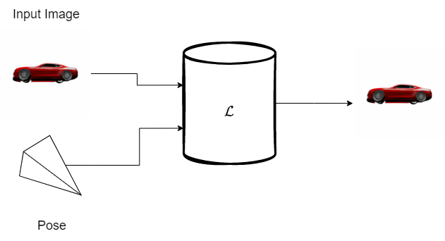
The LFN takes as input a 2D image of a scene and the corresponding camera matrix and outputs a 2D image of the scene for a different point of view.

Camera matrix in this article refers to the $3 \times 4$ matrix that maps 3D world coordinates to 2D coordinates. It is used to convert the 3D points of a scene in the real world, captured by the camera, to a 2D image. There are two camera matrices, the internal and external camera matrices. The external camera matrix is important because the camera coordinate and world coordinate systems might be different. However, I only mention this for completeness, for now all we need to know is that there is a matrix, which we refer to as the pose, that is used to inform the LFN about the orientation of the camera with respect to the scene. If you want to know more about camera matrices, I would like to refer you to the following Image Processing and Computer Vision tutorial.

The LFN parameterizes the Light Field Function for the 2D image and the Light Field Function maps the color to each ray that intersects with the scene (the 2D image). Thus, in order for the LFN to be able to parameterize the Light Field Function, it needs to have access to some more information such as the rays that intersect with the scene, the intersection points of those rays and of course some information about what is displayed in the scene. The LFN relies on an embedding layer which encodes the most important visual information in the image, this is later on used to render the novel view. The part that is responsible for the parameterization of the Light Field function is a multi-layered perceptron (MLP).

I always like to think of an embedding layer as a Lookup Table with weights, where each row corresponds to a sample in our data set and the row contains a weight that describes the characteristics of the sample. In this specific case, if we would use a dataset consisting of images, then each row in the embedding layer is related to a specific image and the row contains the weights that can be used to recreate the image.

Let’s zoom out a bit and reconsider what the LFN actually does. The LFN takes as input a 2D image and the pose corresponding to that image. The pose contains information about the orientation of the camera with respect to the image. The LFN uses an embedding layer to extract visual information about the image and it calculates the rays. Finally, the LFN parameterizes the Light Field function and outputs a novel view of the image.

Figure 1. Simplified overview of the architecture of the LFN

The main question that is left for us to answer is how the LFN calculates the rays and in order to be able to do that we have to explain another concept called the Plücker coordinates. However, before we do so, let’s briefly discuss ray parameterizations. A ray starts at one point, $\mathbf{p}$ and continues forever in a certain direction, $\overset{\rightharpoonup}{v}$ , thus $r = \mathbf{p} + \overset{\rightharpoonup}{v}$. However, this notation is problematic in the sense that it is not unique for a ray.
Let’s imagine we have a ray $r$ that starts at $A$ and goes through $B$, $\overrightarrow{AB}$, in direction $\overset{\rightharpoonup}{v}$. Then we can parameterize the same ray in two ways, $ r = A + \overset{\rightharpoonup}{v}$ or $ r = B + \overset{\rightharpoonup}{v}$, both of these notations refer to the same ray (Figure 2). The problem with this non-uniqueness is that the MLP would have to learn the implicit relation between the different parameterizations for the same rays. The Plücker coordinate notation overcomes this limitation because they are unique for each ray.

Figure 2. Example of a ray

The Plücker notation parameterizes a ray as a tuple of the direction and moment. The moment of a ray is the cross product between any point, $\mathbf{p}$, on the ray and the direction, $\mathbf{d}$, of the ray. The parameterization of the ray $r$ becomes $r = (\mathbf{d}, \mathbf{m}) $, where $\mathbf{m} = \mathbf{p} \times \mathbf{d}$. The key takeaway is that these plücker coordinates are unique for each ray, for more information and proof I would like to refer you to the notes on plücker coordinates by Richard Groff and [1].

Let’s circle back to our main question, “How does the LFN construct the rays and determine the intersection points with the scene?”. We know that the LFN parameterizes the rays with Plücker coordinates and that these are unique for each ray. We also know that the LFN uses the camera matrix to convert from 2D points (pixels) to 3D points. These 3D points are the start points of the ray and what is left to determine is the direction of the ray. In order to obtain the direction of a ray, you can subtract two points that are on that ray. If we consider the ray in figure 2, then in order to get the direction of $r$ we subtract $A$ from $B$, e.g. $\mathbf{d} = A - B$. The LFN does this in the same way by subtracting the coordinates of the camera position from the pixel coordinates. After having obtained the direction, the LFN continues with determining the Plücker coordinates and it uses the camera position as starting point $p$ of the ray, thus $r = \bigl( \mathbf{d}, p \times \mathbf{d} \bigr)$

An interesting observation is that the LFN does not have to do ray tracing, it only requires a single evaluation since the pixel coordinates (which are the intersection points) are already known.

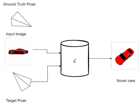
The LFN then continues with the parameterization of the Light Field function and uses it to assign the appropriate color to the ray, after many training iterations the LFN learns to parameterize the Light Field functions that correspond with the input. However, one of the most interesting aspects of the LFN is that it is capable of synthesizing novel views. In figure 3 and 4 we can see an example of what happens during training and testing.

Figure 3. Overview of the task during training. The pose represents the orientation of the camera w.r.t. the scene and the $\mathcal{L}$ represents the Light Field Network.

The LFN is trained to reconstruct the input image, it takes as input a 2D image and the corresponding pose. It then has to parameterize the Light Field function such that it is able to assign the correct colors to the calculated rays. It also uses the visual information encoded by the Embedding layer to assign the colors to the rays.

Figure 4. Overview of the task during testing. The pose represents the orientation of the camera w.r.t. the scene. In this case, the pose does not correspond to the input image but should correspond to the output image. The Light Field Network, represented as $\mathcal{L}$, should synthesize the novel view that corresponds to the pose.

During testing, the LFN is given a pose (camera matrix) that does not correspond to the camera matrix of the input. The LFN has to synthesize this new view by parameterizing the Light Field function that actually corresponds to the given camera matrix, this is also called novel view synthesis.

Extracting Geometry from the LFN

The last thing I would like to discuss about the LFN is the fact that they can be used to extract point clouds and depth maps. If you have the Light Field function of a scene then you also have the information necessary to reconstruct the depth of the scene. However, this information is not always straightforward to extract because the parameterization of the Light Field as explained in one of my earlier post considers the image projected onto a plane with cartesian coordinates $x,y$. It is therefore not straightforward to infer the depth.

Fortunately, in the case of the LFN, there is a certain assumption that introduces certain properties that allow for extraction of depth from the Light Field function.

Lambertian Reflection

Since the LFN builds upon the Light Field and the Lumigraph, we have the restriction that the color of a ray should not change. The underlying assumption is that there is no dispersion of light and that light is reflected equally in all directions, this is also referred to as Lambertian Reflection (Figure 5).

Figure 5. overview of the different types of reflection, taken from [2].

In settings where the reflection is Lambertian, the color of a pixel is always consistent along the different viewpoints. In other words, if we would observe a red pixel on a sphere, then that pixel should always be red, regardless of our point of view. The fact that the LFN only works in settings where the reflection is Lambertian is actually one of its limitations. However, it also introduces the possibility to extract depth information quite easily, but before we continue we need to introduce another concept called Epipolar Plane Image (EPI).

Epipolar Plane Imaging

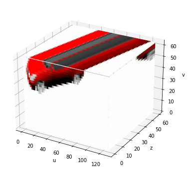
I will briefly introduce EPI such that you can follow along with the rest of this article. If you are interested in learning more about EPIs, I would like to refer you to one of my other posts where we explain both the theory and showcase some code to create our own EPIs. An Epipolar plane image is a volume of images of a static scene recorded by a moving observer (camera). The images are then stacked to form a volume and if we slice through the top of the volume at a certain height, we can see two things; the color of pixels over time and we can deduce depth information due to parallax (Figures 7 and 8). The last one is especially interesting since we are trying to extract information about geometry from the Light Field Function.

Figure 7. EPI

Figure 8. Overview of the top of a sliced through EPI

Before we continue, I would like to stress that the explanation, a more formal one, of extracting geometry information from EPIs and Light Field functions can be found in [1]. However, I struggled with the explanation in the sense that it was quite abstract and concise. I will therefore try to provide a simpler explanation, which helped me understand the concept. First, I will provide the equation from the article ( eq. \ref{eq:depth_extraction} from [1]), explain the terms in the equation and then continue to explain how it relates to extracting geometry from EPIs.

\begin{equation} \begin{split} \mathbf{c}\bigl(s,t\bigr) & = \Phi\bigl(\mathbf{r}\bigl(s,t\bigr)\bigr) \\
\text{where } \mathbf{r}\bigl(s,t\bigr) & = \overrightarrow{\mathbf{a}\bigl(s\bigr)\mathbf{b}\bigl(t\bigr)} \\
& = \Biggl(\frac{\mathbf{b}\bigl(t\bigr) - \mathbf{a}\bigl(s\bigr)} {\big\|\mathbf{b}\bigl(t\bigr) - \mathbf{a}\bigl(s\bigr)\big\|}, \frac{\mathbf{a}\bigl(s\bigr)\times\mathbf{b}\bigl(t\bigr)} {\big\|\mathbf{b}\bigl(t\bigr) - \mathbf{a}\bigl(s\bigr)\big\|}\Biggr) \end{split} \tag{1} \label{eq:depth_extraction} \end{equation}

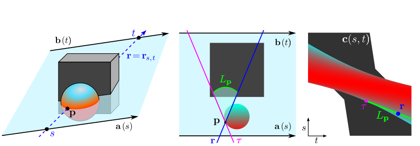
First, we go over the definitions of the terms and what they represent and then we will circle back and try to see the bigger picture and how everything relates. The figures in Figure 9 are helpful in understanding what is meant by certain terms in equation \ref{eq:depth_extraction}, the figure is copied from the paper on Light Field Networks [1].

Figure 9. Visualization of how depth is extracted from EPIs, taken from [1]

The order in which we go over the terms in the equation might be confusing initially but in the end it will make sense (hopefully).

Let’s go over the first part $\mathbf{c}\bigl(s,t\bigr)$, it has parameters $s$ and $t$. In the left most figure in figure 9, a ray $\mathbf{r}$ and two rays $\mathbf{b}\bigl(t\bigr)$ and $\mathbf{a}\bigl(s\bigr)$ are displayed. First, we pick two points, $x,x’ \in \mathbb{R}^3$, that lie on on $\mathbf{r}$, then we parameterize two rays that are orthogonal to $r$ and intersect with these points, which are called $s$ and $t$. The rays $\mathbf{a}\bigl(s\bigr) = \bigl(x + s\mathbf{d}\bigr)$ and $\mathbf{b}\bigl(t\bigr)=\bigl(x’ + t\mathbf{d}\bigr)$, are parallel to eachother and orthogonal to $\mathbf{r}$. They form a 2D plane $(s,t)$ in which a group of rays lie, or in other words, this is the 2D parameterization of a Light Field. This group of rays is represented by the term $\mathbf{c}\bigl(s,\bigr)$ and the colors for those rays are determined by the LFN $\Phi\biggl(\mathbf{r}\bigl(s,t\bigr)\biggr)$.

Let’s say we are interested in point $\mathbf{p}$, e.g. we would like to extract depth information with respect to point $\mathbf{p}$. We have a 2D Light Field and what we can do now is draw all rays that pass through point $\mathbf{p}$, this is visualized in the middle subfigure of figure 9. The magenta line $\tau$ is the last line that intersects with point $p$, and between the ray $\mathbf{r}$ and point $\tau$ lies a family of rays that go through $\mathbf{p}$. An important thing is to keep in mind that all these, non occluded rays, must have the same color (remember Lambertian Reflection). If we draw all rays in this Light Field and then plot the color of the ray, then we obtain the EPI (right most figure of figure 9). In the gif in figure 10, an example of what is meant by drawing all the rays in a light field and then plotting the colors of those rays is shown.

Figure 10. Example of how the EPI is created by plotting all the colors of the rays in a Light Field, taken from [3]

Let’s reiterate the steps we took, we created two rays $\mathbf{a}$ and $\mathbf{b}$, parallel to eachother but orthogonal to $\mathbf{r}$, which form a plane ( the 2D Light Field). In this plane we sample all rays and for each ray we plot it’s color, which results in the EPI. Furthermore, let’s re-examine equation \ref{eq:depth_extraction}, where we state that for a family of rays the colors can be determined using the LFN, i.e. $\mathbf{c}\bigl(s,t\bigr) = \Phi\biggl(\mathbf{r}\bigl(s,t\bigr)\biggr)$. The second part of equation \ref{eq:depth_extraction} is quite straightforward, it is a general description of the rays in the Light Field of the 2D plane $(s,t)$. Before we continue with explaining the last part of the equation, I would like to point out that the rays in the plane $(s,t)$ start on $\mathbf{a}\bigl(s\bigr)$ and go through $\mathbf{b}\bigl(t\bigr)$, thus a ray can be parameterized by two points, one on $\mathbf{a}$ and one on $\mathbf{b}$. The first part; $\frac{\mathbf{b}\bigl(t\bigr) - \mathbf{a}\bigl(s\bigr)} {\big\|\mathbf{b}\bigl(t\bigr) - \mathbf{a}\bigl(s\bigr)\big\|}$, is thus the normalized direction. The second part; $\frac{\mathbf{a}\bigl(s\bigr)\times\mathbf{b}\bigl(t\bigr)} {\big\|\mathbf{b}\bigl(t\bigr) - \mathbf{a}\bigl(s\bigr)\big\|}$, is a normalized vector, normal to the plane formed by the lines $\mathbf{a}\bigl(s\bigr)$ and $\mathbf{b}\bigl(t\bigr)$.

We know that the Plücker parameterization of a ray is $\mathbf{r}\bigl(\mathbf{d}, \mathbf{m}\bigr)$ where $\mathbf{d}$ is the direction and $\mathbf{m}$ is the moment. The moment is a vector where its magnitude represents the distance between the origin of a ray and a plane that can be formed between the ray and the origin of the ray. In our case, the origin of the ray is on $\mathbf{a}\bigl(s\bigr)$ and it resides in the 2D plane formed by $\mathbf{a}\bigl(s\bigr)$ and $\mathbf{b}\bigl(t\bigr)$. Thus the second element of the tuple in equation \ref{eq:depth_extraction} can be characterized as the moment.

In other words, the two elements of the tuple in \ref{eq:depth_extraction} is the Plücker parameterization of ray $\mathbf{r}\bigl(s,t\bigr)$.

Now that we understand how the Light Field is constructed and how the EPI is constructed from the Light Field, we can continue with exploring how depth is extracted from the EPI. The first thing we should notice is that the family of rays that pass through $\mathbf{p}$ are represented as $L_p$ in figure 9. If we draw the EPI points for all the rays in $L_p$ we notice that they are on a line (Figures 9 and 10), and since we are dealing with Lambertian reflection the colors of these points should be the same. However, the most interesting aspect is that if we pick a point closer to the camera $\mathbf{p’}$ and construct a new family of rays, $L_{p’}$, that go through that point, then we can use the gradient of the lines to obtain information about the depth of those points (Figure 11).

Figure 11. Overview of how different families of rays through different points in the scene, have a different slope. This information is used in extracting geometry of a scene. Taken from [3]

In the paper, they show how we can use the distance between $\mathbf{a}\bigl(s\bigr)$ and $\mathbf{b}\bigl(t\bigr)$ and the gradient of the slope for the family of rays $L_p$ to calculate the depth of point $\mathbf{p}$. However, we now understand the background information required to follow along with the proposition and proofs explained in [1], so I would like to refer you to [1] in case you are interested in the exact methodology.

The code for extracting depth maps and point clouds can be found on my github as well as a jupyter notebook that you can run. All instructions for running the code can be found in the readme of the github repository.

In conclusion, we have discussed the Light Field Network and its relation to Light Field functions. We have also explained how geometry information can be extracted from the EPI which can be constructed by sampling rays in a Light Field. Finally, the links to the code in my github repository should be useful in case you would like to tinker around with the LFN. As always, feedback is very welcome, feel free to point out any flaws, errors, other interesting things or parts that need more clarification.

References

[1] Vincent Sitzmann, Semon Rezchikov, William T. Freeman, Joshua B. Tenenbaum, and Fredo Du- rand. Light field networks: Neural scene representations with single-evaluation rendering. 6 2021.

[2] https://notebook.community/tensorflow/graphics/tensorflow_graphics/notebooks/reflectance

[3] https://papertalk.org/papertalks/37418